while(motivation <= 0)

6/13/2026
- [ ] Drivable golf cart
- [ ] Hand animation for turning golf cart wheel
- [ ] vegetation generator bound to mesh
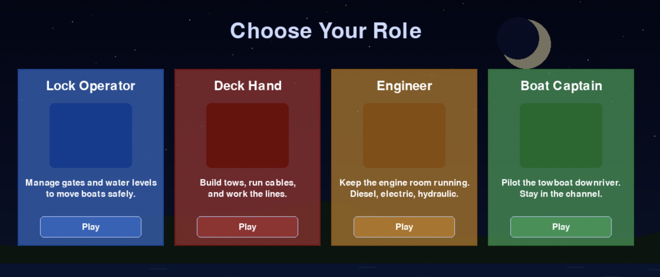
- [ ] game type menu for story or freeplay mode
- [ ] Building out the operator home
- [ ] Operator able to set on chairs without hands in driving hands
- [ ] New assets
    - [ ] Golf Cart
    - [ ] Trees, Bushes, Weeds, Flowers
    - [ ] House stuff, houses
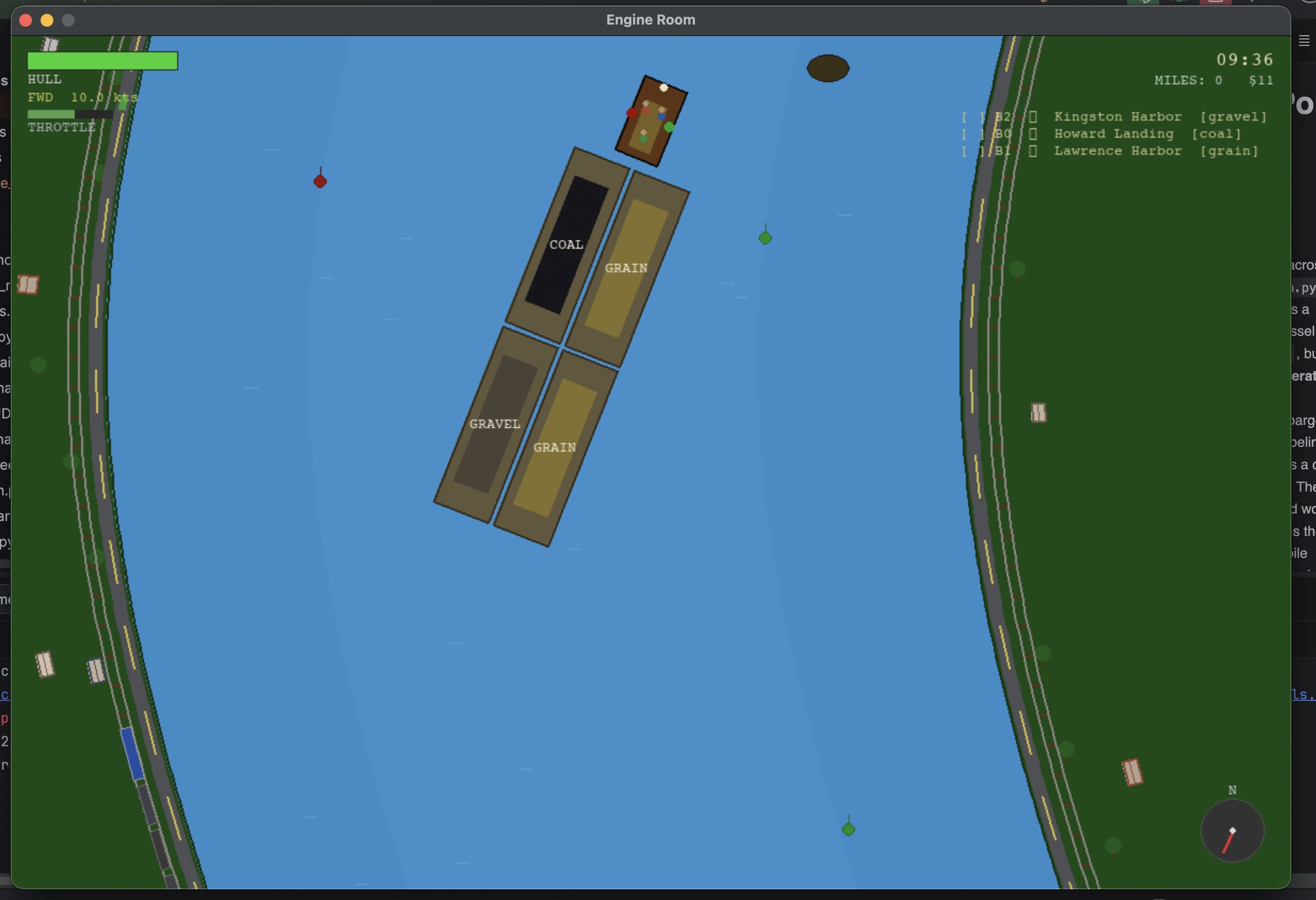
- [ ] Procedurally generated river, started work on “deck hand” scene.
- [ ] Menu fixes

6/19/2026
- [ ] Tope tie off mini game
- [ ] bug fixed walking, running, flowing down river
- [ ] drowning prototype
- [ ] river boats turning naturally
- [ ] river boats spawning with variety
- [ ] river boats avoiding tow / barges
- [ ] fixed trees spawning on proc river
- [ ] water not bleeding through barges
- [ ] player not drowning while in barge
- [ ] tested paid version of meshy.ai; models look good from a distance, up close they are quite rough.

6/29/2026
- [ ] Rewrote the beginning of the story.
- [ ] Meshy.ai model of a great blue heron

Highlights from this weekend in GBH:

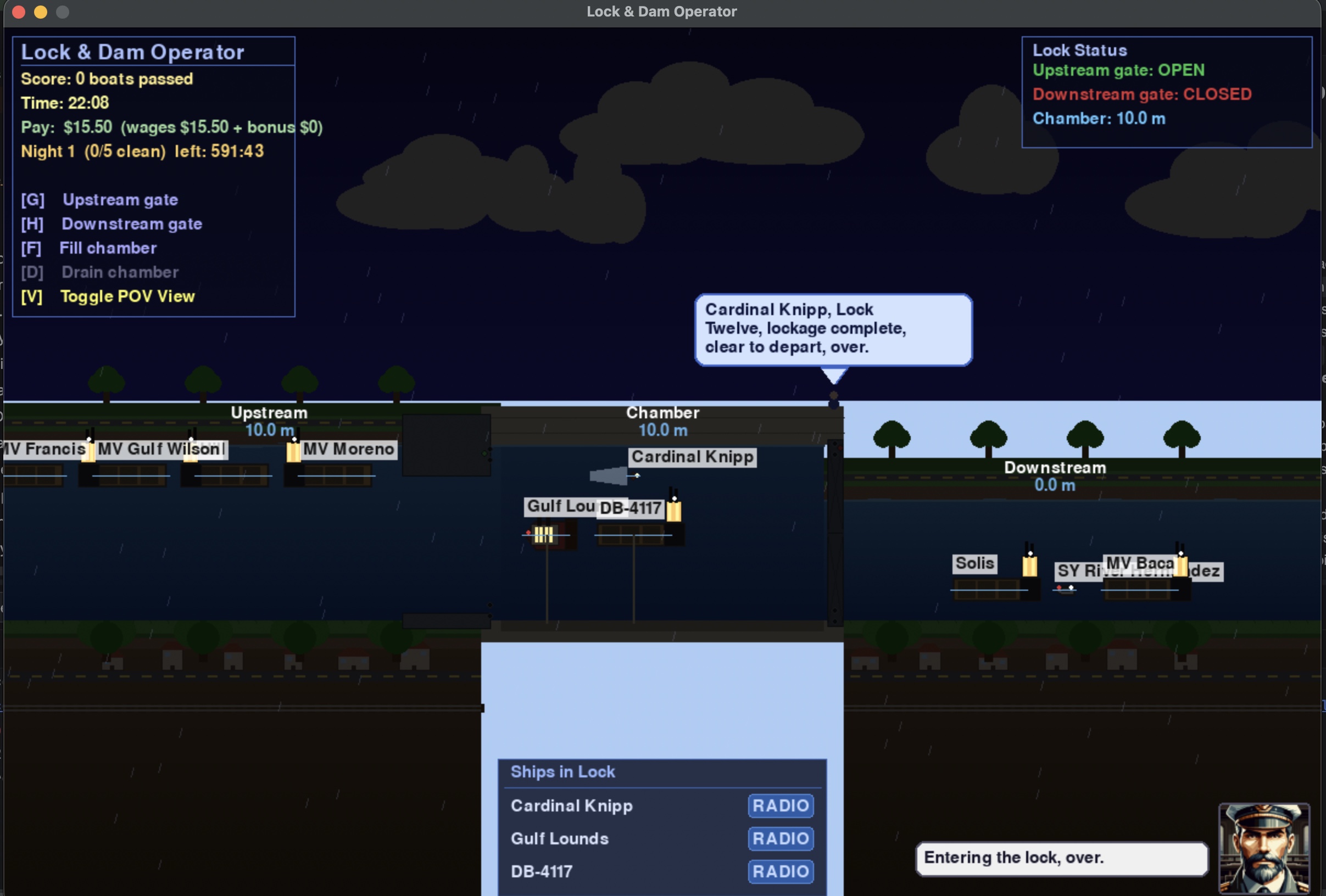
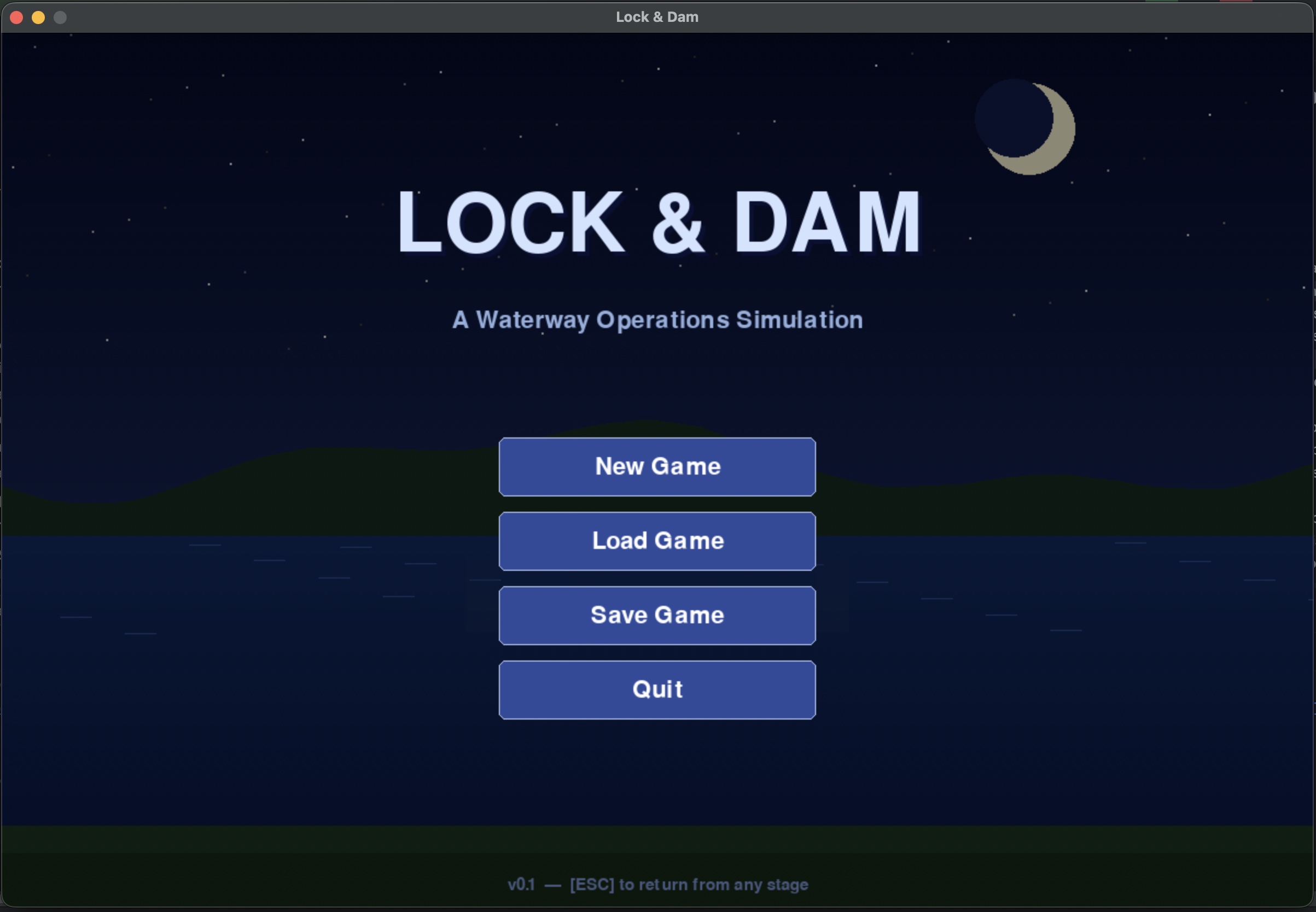
- [ ] HDR Water (mostly)
- [ ] Fixed cameras for HDR
- [ ] Added boat colors into boat spawn arrays
- [ ] Added a Continue Game button to the menu
- [ ] Started writing prolog, and night one in Inkly
- [ ] boats not passing through each other, but going off like boats would
- [ ] modeled radio, added knobs, power light, power switch, mic, speaker
- [ ] radio-controlled traffic from the control room, a work in progress. Still a bit buggy.

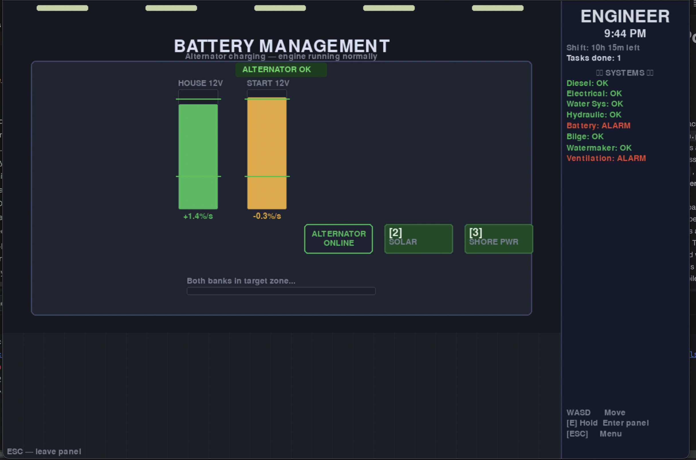
interactable doors
turning control knobs that interact with the world
control lever
Room and door modeling on the Tow Boat
working Security camera feeds
Control room readouts with sim data, like water level.
Moved the operator start point to the control room
Tow + Barge spawn and layout control for lock traffic

It was a three-day holiday weekend, so a lot of progress was made.

• Operator 3d movement
• Operator 3rd person follow mode
• Operator first-person view with fly and no clip when in dev mode.
• Operator walk/run animations and speed
• Operator physics/clipping on objects
• World scale adjustments to match the operator
• Unity store asset integration of recreational boats
• Started modeling tow-boat and flat front barges
• Started writing story player dialog trees

I like the notion of having the dialog choices that the player chooses steer their archetype.

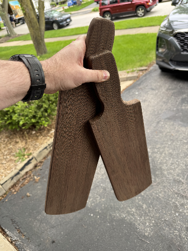
This weekend was a healthy mix of online and IRL. After doing some grocery shopping and hitting the range on Saturday, I set out to make some drink flight boards for the mother-in-law. She hasn’t picked out any glasses for them yet, so once she does that, I’ll fix some less-than-cementary features and cut holes for the glasses to sit on.

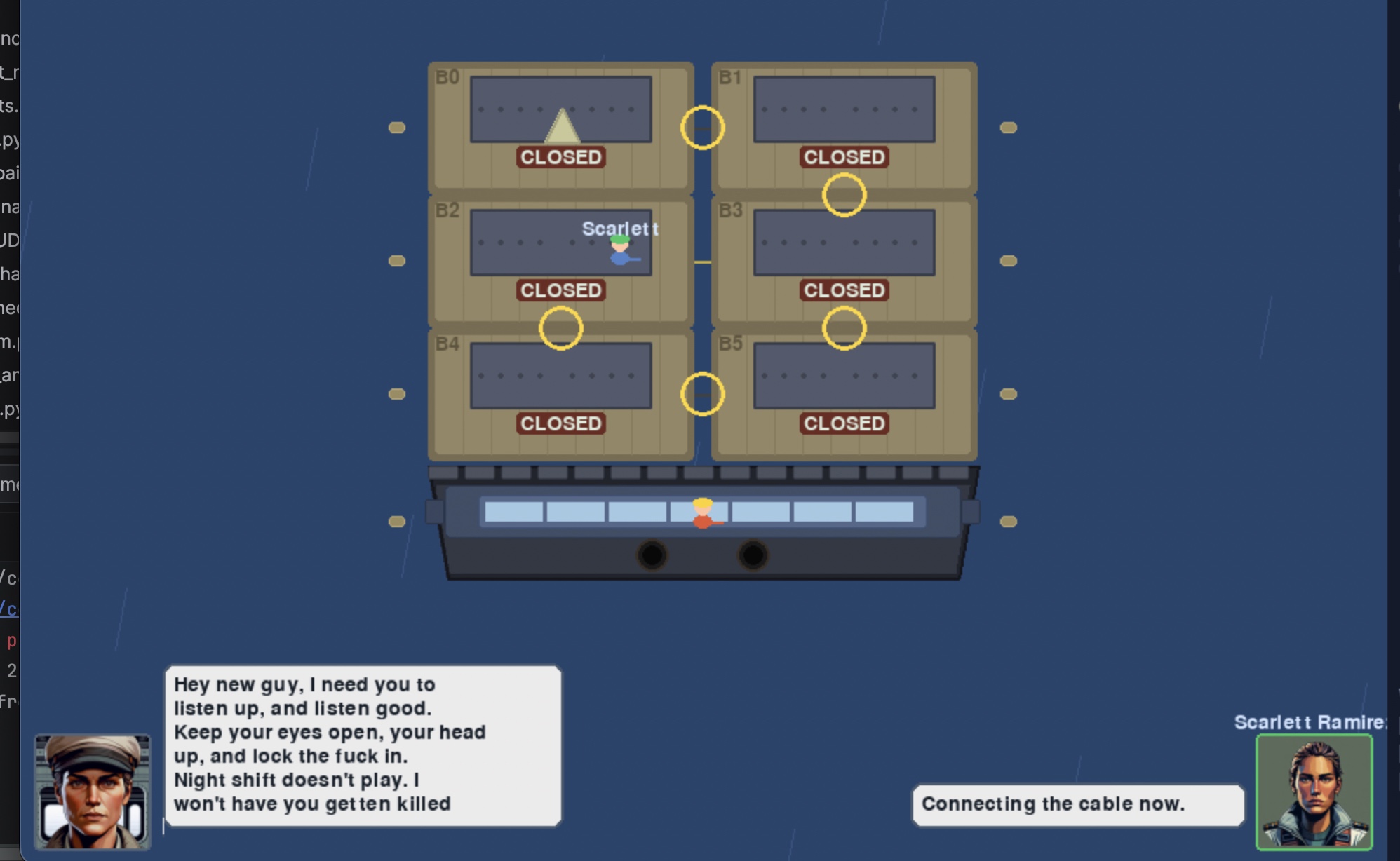
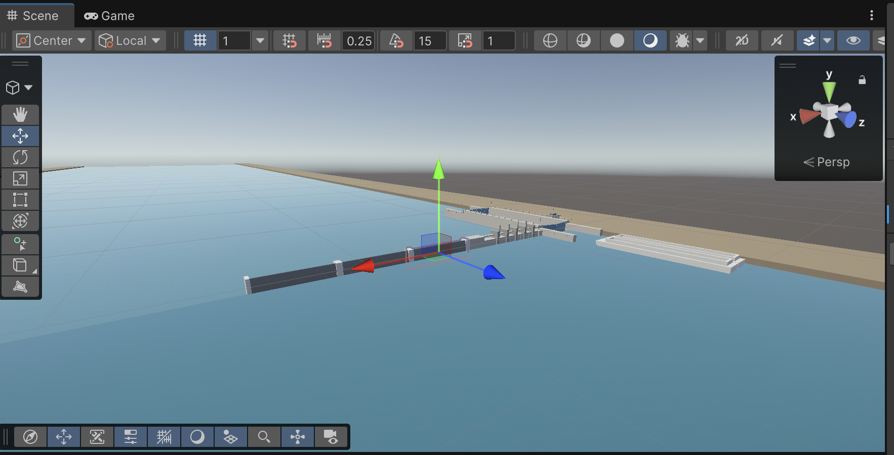
The next phase of the weekend was picking up my Unity project to build out my Python game Project Albatross and build out the functionality into Unity. This all went quite a bit better than I would have expected, and I’ve been making steady progress. While we sorted the menu last weekend, this weekend I implemented the simulation engine parts from the other project, modeled some lock gates, and got the lock gate animation working. It’s surprisingly difficult to get Claude to implement how doors work in 2d or 3d space. We got through it, but it took most of Sunday to work out the kinks. I also decided to invest in a premade lock worker model. She looks decent and fits the cartoonish look I had in mind.

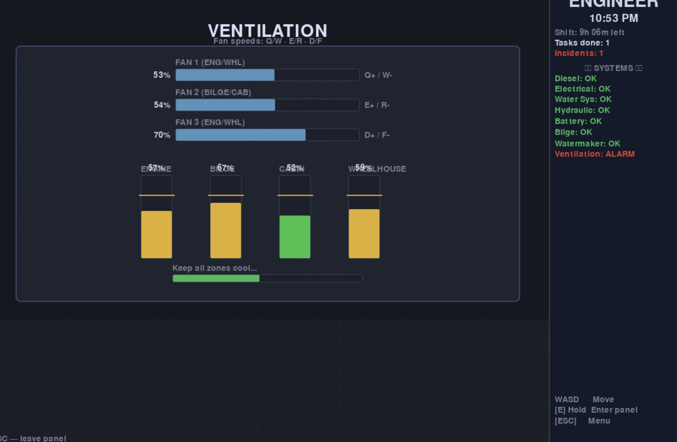
I spent most of the weekend testing Claude's ability to generate Unity assets in Blender. As it turns out, it does a decent enough job. So when my hands had had enough of Blender and Unity, I went back to Albatross and did some work on the deck-hand sim, came up with a couple of new games, and did a bunch of enhancements.

One weekend, while I was working on finishing up my open port of Second Conflict, I was away from my intel laptop and picked up project Albatros.

Project Albatros was a little thought experiment that I started in October of 2025, using Amazon Q to see if I could build a lock and dam simulator. I have fond memories from my childhood at a children's center playing with a lock and dam system toy with moving water, gates, and pumps. It was the highlight of my day after spending the rest of the day walking around with my parents at an art show. As a Boy Scout, we also visited and got a tour of one of the locks and dams on the Mississippi River. It was running on a mainframe that took up an entire wall in the building next to the lock. Walking across the gates with high waves was also a bit terrifying as a kid.

I’ve been fairly impressed using Anthropic Claude to crank through software projects and make my creative ideas come to life without days of coding that cause a lot of wear on my old (Nintendo-damaged) hands. I was mostly delighted to see Claude really bring my ideas to life, and I quickly burned through my token allowance.

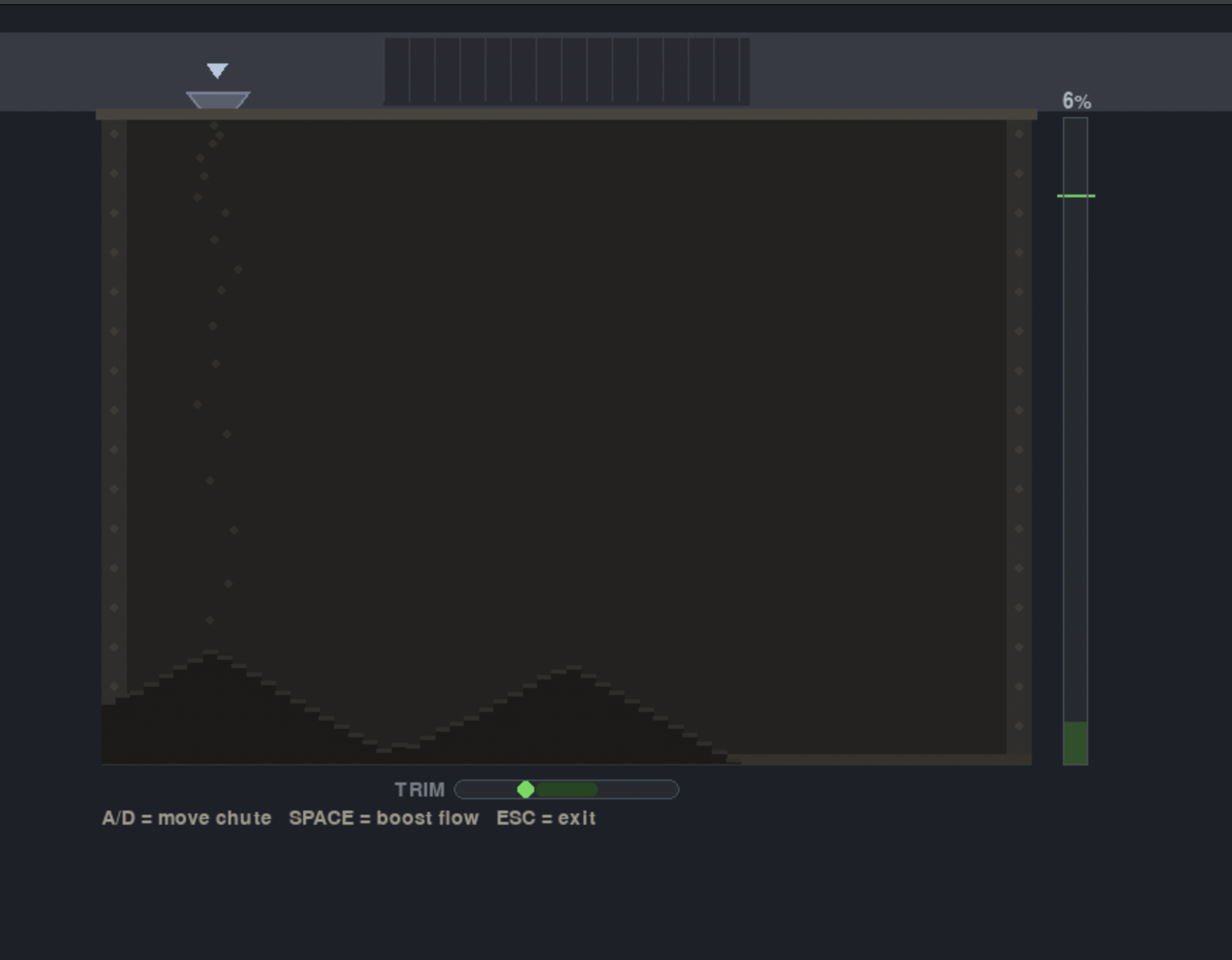
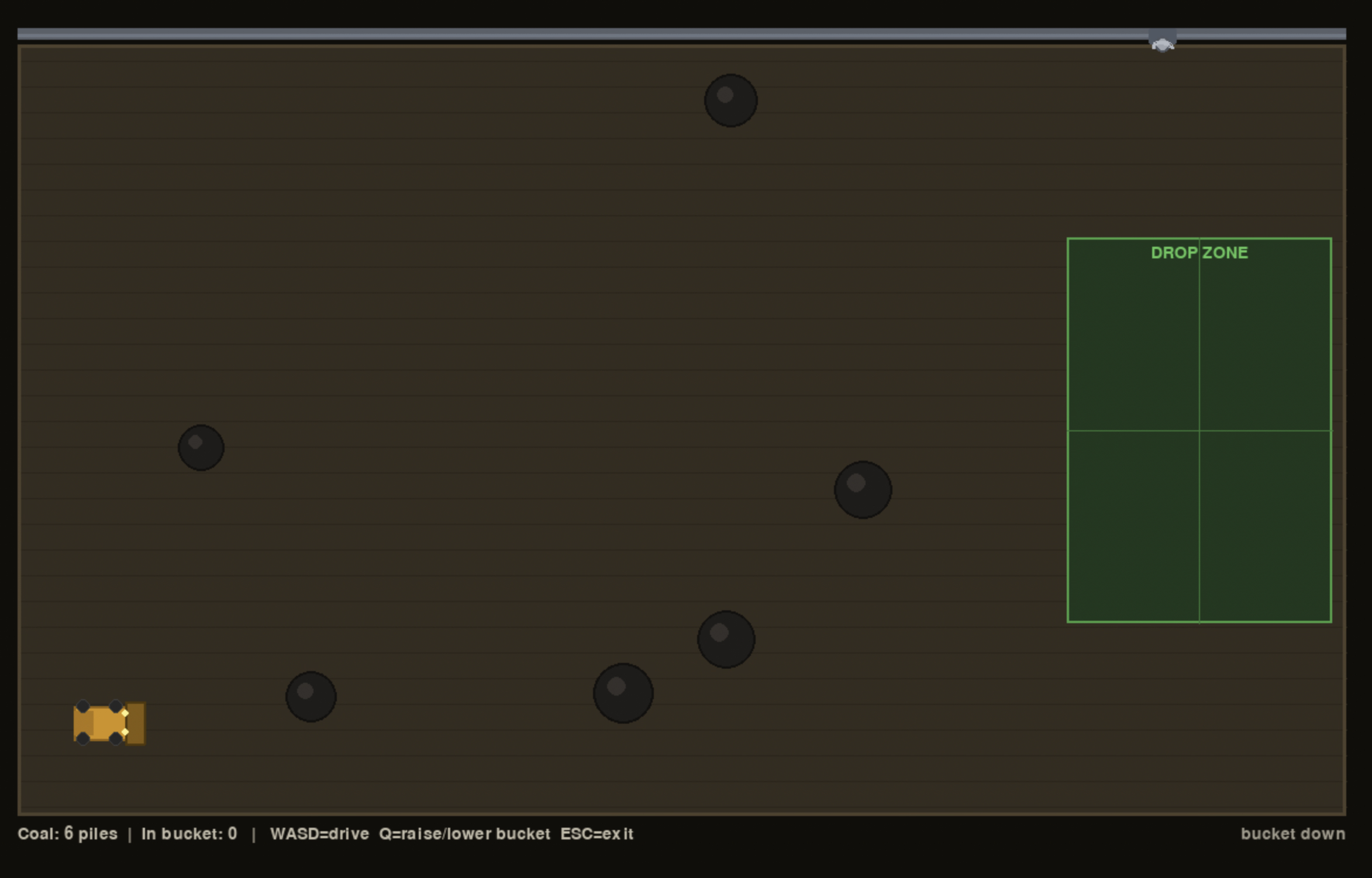
Once I had the lock and dam sim to a decent working state, I started daydreaming about other waterway-related games and how I could tie them all together. So I’ve spent the month of April building games and mini-games in Python Pygame. The results look like something out of the early 90s, and I can’t help but think that while I really enjoy working with Python, PyGame is holding me back from the bigger aspirations I have for the game. A lot of things I want to implement are clunky to do.